Community analysis

Overview

Code

Y_fitted_H1 <- readRDS(here_rel("results", "models", "H1", "Y_H1_fitted.rds")) |>
  sf::st_transform("EPSG:32622")

Y_fitted_H1 <- Y_fitted_H1 |> mutate(X_utm = st_coordinates(Y_fitted_H1)[,1], 
Y_utm = st_coordinates(Y_fitted_H1)[,2]) |> sf::st_drop_geometry()

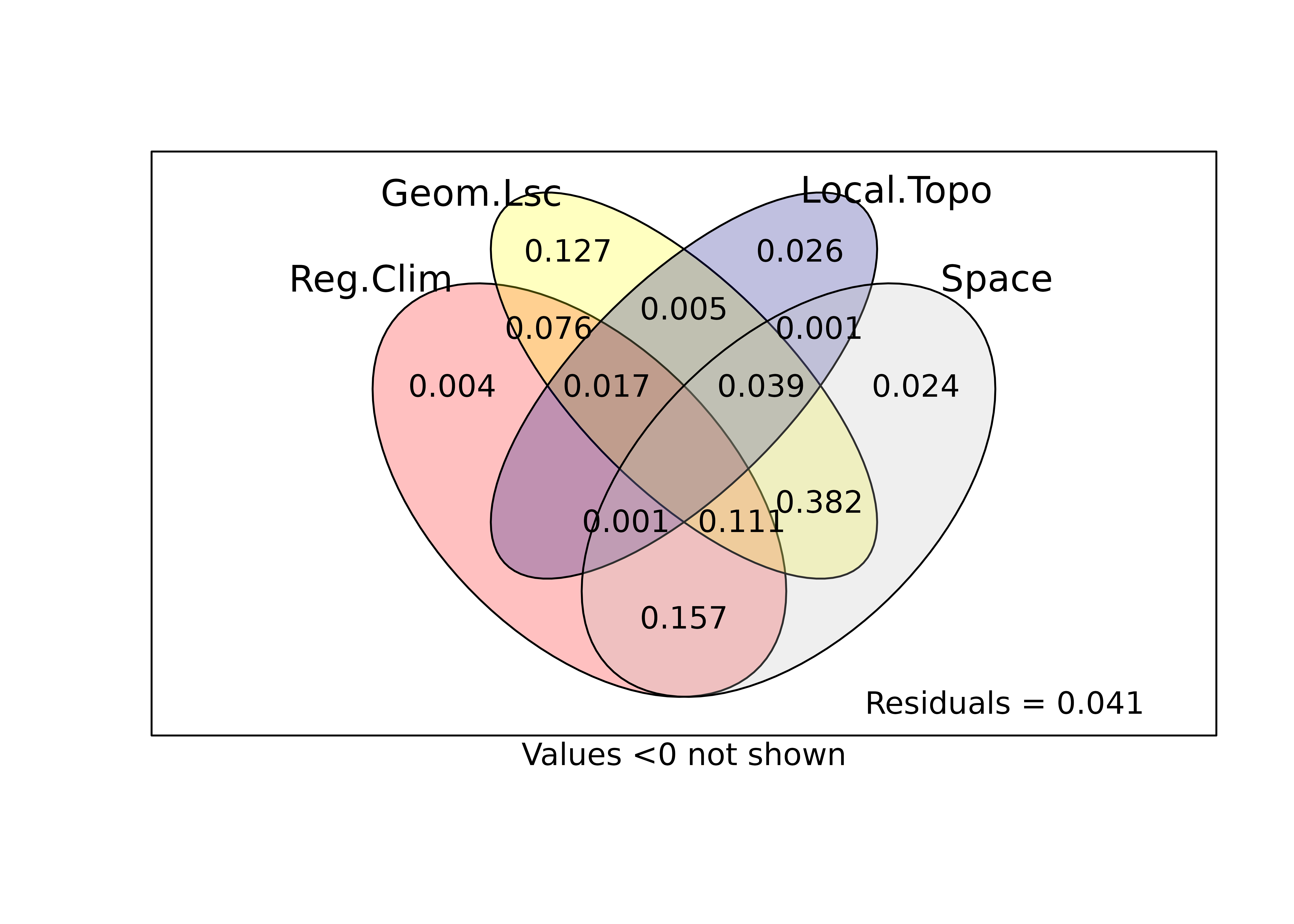
This section quantifies how much variation in community composition is attributable to (i) regional climate, (ii) geomorphological subtypes, and (iii) local topography (SWI), and how these fractions change once spatial structure is made explicit. We report variance partitioning both without and with spatial predictors, to distinguish “pure environmental” effects from components that are environmentally structured in space or confounded with dispersal limitation.

We use the model-based fitted community matrix (Dirichlet–multinomial draws or posterior mean composition), converted to relative abundances and analysed with redundancy analysis (RDA) variance partitioning.

Code

#|code-fold: true

# Community matrix: relative abundance (rows = sites, cols = species)
comm <- Y_fitted_H1$Y_fit_mean / rowSums(Y_fitted_H1$Y_fit_mean)

# Environmental blocks
X_clim <- scale(Y_fitted_H1[, c("Clim1", "Clim2")])
X_geom <- Y_fitted_H1[, c("GeomSub")]
X_swi  <- scale(log(Y_fitted_H1[, c("SWI")] + 1))

Variance partitioning without spatial structure

Code

if (!file.exists(
    here_rel("results", "models", "H1", "varpart_H1.rds")
)) {
    varpart_env <- vegan::varpart(
    Y = comm, transfo = "total",
    X_clim, X_geom, X_swi
  )
  saveRDS(varpart_env, here_rel("results", "models", "H1", "varpart_H1.rds"))
}else{
  varpart_env <- readRDS(here_rel("results", "models", "H1", "varpart_H1.rds"))
}

plot (varpart_env, digits = 2, Xnames = c('Reg.Clim', 'Geom.Lsc','Local.Topo'), 
bg = c('red', 'yellow','navy'))

The “pure” fractions represent variation uniquely explained by each block once the other two blocks are controlled for. Shared fractions represent overlap among blocks, i.e. environmental covariation that makes contributions statistically inseparable at the community level.

SI: Multi-scale spatial pattern analysis

To estimate the unique environmental effects decoupled from spatial effects, we used Principal Coordinates of Neighbourhood Matrix - PCNM (Stéphane Dray, Legendre, and Peres-Neto (2006); S. Dray et al. (2012)) to visualize and quantify multiscale spatial autocorrelation in community composition. The procedure (i) computes the spatial distance matrix among inventory units centroids which define the graph where the nodes are the plots; (ii) defines a truncation threshold $d_0$ equal to the longest edge of the minimum spanning tree (MST), ensuring graph connectivity; (iii) constructs a weighted neighborhood matrix $W$ with $W_{ij}=1-\dfrac{d_{ij}}{d_0}$ if $d_{ij}<d_0$ ($W_{ij}=0$ otherwise); and (iv) performs a principal coordinates analysis on the truncated distance matrix to obtain orthogonal eigenvectors (PCNM variables). Each eigenvector represents a sinusoidal spatial pattern at a characteristic scale, from broad (leading vectors) to fine (higher-order vectors), and its spatial relevance is assessed by Moran’s $I$ computed with $W$. Following standard recommendations, we retained only eigenvectors with positive autocorrelation (Moran’s $I>0$), which capture aggregation patterns.

Code

if (!file.exists(
    here_rel("results", "models", "H1", "pncm_H1.rds")
)) {
      
  pcnm_H1 <- vegan::pcnm(dist(Y_fitted_H1[,c("X_utm", "Y_utm")]) / 1E3)
  saveRDS(pcnm_H1, here_rel("results", "models", "H1", "pncm_H1.rds"))
}else{
  pcnm_H1 <- readRDS(here_rel("results", "models", "H1", "pncm_H1.rds"))
}

if (!file.exists(
    here_rel("results", "models", "H1", "varpart_sp_H1.rds")
)) {
    varpart_sp <- vegan::varpart(
    Y = comm, transfo = "total",
    X_clim, X_geom, X_swi,pcnm_H1$vectors
  )
  saveRDS(varpart_sp, here_rel("results", "models", "H1", "varpart_sp_H1.rds"))
}else{
  varpart_sp <- readRDS(here_rel("results", "models", "H1", "varpart_sp_H1.rds"))
}

plot(varpart_sp, 
  digits = 2, 
  Xnames = c('Reg.Clim', 'Geom.Lsc','Local.Topo','Space'), 
  bg = c('red', 'yellow','navy',"grey75")
  )

Side-by-side comparison: without vs with space

Code


# Helper to extract the three pure fractions from a 3-block varpart object
    pure3 <- function(vp){
      tibble(
        Climate = vp$part$indfract[1, "Adj.R.square"],
        Geomorphology = vp$part$indfract[2, "Adj.R.square"],
        LocalTopography = vp$part$indfract[3, "Adj.R.square"]
      )
    }

pure_env <- pure3(varpart_env) |>
      pivot_longer(everything(), names_to = "block", values_to = "adjR2") |>
      mutate(model = "Environment only")

pure_env_space <- tibble(
      Climate = varpart_sp$part$indfract[1, "Adj.R.square"],
      Geomorphology = varpart_sp$part$indfract[2, "Adj.R.square"],
      LocalTopography = varpart_sp$part$indfract[3, "Adj.R.square"],
      Space = varpart_sp$part$indfract[4, "Adj.R.square"]
    ) |>
      pivot_longer(everything(), names_to = "block", values_to = "adjR2") |>
      mutate(model = "Environment + space")

bind_rows(pure_env, pure_env_space) |>
      mutate(adjR2 = round(adjR2, 4)) |>
      arrange(block) |>
      knitr::kable(caption = "Pure adjusted R² fractions without vs with an explicit spatial block (PCNM).")

Pure adjusted R² fractions without vs with an explicit spatial block (PCNM).
block	adjR2	model
Climate	0.161	Environment only
Climate	0.004	Environment + space
Geomorphology	0.509	Environment only
Geomorphology	0.127	Environment + space
LocalTopography	0.027	Environment only
LocalTopography	0.026	Environment + space
Space	0.024	Environment + space

When adding space reduces the pure environmental fractions, the difference indicates that part of the apparent environmental signal is spatially structured—either because environmental gradients themselves are spatially organised (e.g. regional climate gradients), or because unmeasured spatial processes (dispersal limitation, historical contingencies) co-vary with the measured environment.

In ecological terms, the “environment ∩ space” component should not be interpreted as purely neutral: it can reflect both genuine environmental filtering expressed along spatially structured gradients and spatial processes not captured by the predictors. The remaining “pure environment” fractions represent the most conservative estimate of scale-specific filtering that is statistically separable from space.

References

Dray, S., R. Pélissier, P. Couteron, M.-J. Fortin, P. Legendre, P. R. Peres-Neto, E. Bellier, et al. 2012. “Community Ecology in the Age of Multivariate Multiscale Spatial Analysis.” Ecological Monographs 82 (3): 257–75. https://doi.org/10.1890/11-1183.1.

Dray, Stéphane, Pierre Legendre, and Pedro R. Peres-Neto. 2006. “Spatial Modelling: A Comprehensive Framework for Principal Coordinate Analysis of Neighbour Matrices (PCNM).” Ecological Modelling 196 (3): 483–93. https://doi.org/10.1016/j.ecolmodel.2006.02.015.

--- title: "Community analysis" format: html: code-fold: true --- ```{r setup, warning=FALSE, message=FALSE, include=FALSE} knitr::opts_chunk$set( fig.align = "center", fig.retina = 3, fig.width = 7, fig.height = 5, out.width = "85%", collapse = TRUE, dev = "ragg_png", warning = FALSE, message = FALSE ) options(digits = 3, width = 120, dplyr.summarise.inform = FALSE) set.seed(1234) here_rel <- function(...) { fs::path_rel(here::here(...)) } ``` ```{r libraries-data, warning=FALSE, message=FALSE, include=FALSE} library(tidyverse) library(vegan) library(eulerr) library(adespatial) library(sf) source(here_rel("R", "funs_data.R")) source(here_rel("R", "funs_graphics.R")) source(here_rel("R", "funs_plot_tables.R")) theme_set(theme_public()) ``` # Overview ```{r} Y_fitted_H1 <- readRDS(here_rel("results", "models", "H1", "Y_H1_fitted.rds")) |> sf::st_transform("EPSG:32622") Y_fitted_H1 <- Y_fitted_H1 |> mutate(X_utm = st_coordinates(Y_fitted_H1)[,1], Y_utm = st_coordinates(Y_fitted_H1)[,2]) |> sf::st_drop_geometry() ``` This section quantifies how much variation in community composition is attributable to (i) regional climate, (ii) geomorphological subtypes, and (iii) local topography (SWI), and how these fractions change once spatial structure is made explicit. We report variance partitioning both without and with spatial predictors, to distinguish “pure environmental” effects from components that are environmentally structured in space or confounded with dispersal limitation. We use the model-based fitted community matrix (Dirichlet–multinomial draws or posterior mean composition), converted to relative abundances and analysed with redundancy analysis (RDA) variance partitioning. ```{r} #|code-fold: true # Community matrix: relative abundance (rows = sites, cols = species) comm <- Y_fitted_H1$Y_fit_mean / rowSums(Y_fitted_H1$Y_fit_mean) # Environmental blocks X_clim <- scale(Y_fitted_H1[, c("Clim1", "Clim2")]) X_geom <- Y_fitted_H1[, c("GeomSub")] X_swi <- scale(log(Y_fitted_H1[, c("SWI")] + 1)) ``` ## Variance partitioning without spatial structure ```{r} if (!file.exists( here_rel("results", "models", "H1", "varpart_H1.rds") )) { varpart_env <- vegan::varpart( Y = comm, transfo = "total", X_clim, X_geom, X_swi ) saveRDS(varpart_env, here_rel("results", "models", "H1", "varpart_H1.rds")) }else{ varpart_env <- readRDS(here_rel("results", "models", "H1", "varpart_H1.rds")) } plot (varpart_env, digits = 2, Xnames = c('Reg.Clim', 'Geom.Lsc','Local.Topo'), bg = c('red', 'yellow','navy')) ``` The “pure” fractions represent variation uniquely explained by each block once the other two blocks are controlled for. Shared fractions represent overlap among blocks, i.e. environmental covariation that makes contributions statistically inseparable at the community level. # SI: Multi-scale spatial pattern analysis To estimate the unique environmental effects decoupled from spatial effects, we used Principal Coordinates of Neighbourhood Matrix - PCNM (@draySpatialModellingComprehensive2006; @drayCommunityEcologyAge2012) to visualize and quantify multiscale spatial autocorrelation in community composition. The procedure (i) computes the spatial distance matrix among inventory units centroids which define the graph where the nodes are the plots; (ii) defines a truncation threshold $d_0$ equal to the longest edge of the minimum spanning tree (MST), ensuring graph connectivity; (iii) constructs a weighted neighborhood matrix $W$ with $W_{ij}=1-\dfrac{d_{ij}}{d_0}$ if $d_{ij}<d_0$ ($W_{ij}=0$ otherwise); and (iv) performs a principal coordinates analysis on the truncated distance matrix to obtain orthogonal eigenvectors (PCNM variables). Each eigenvector represents a sinusoidal spatial pattern at a characteristic scale, from broad (leading vectors) to fine (higher-order vectors), and its spatial relevance is assessed by Moran’s $I$ computed with $W$. Following standard recommendations, we retained only eigenvectors with positive autocorrelation (Moran’s $I>0$), which capture aggregation patterns. ```{r} if (!file.exists( here_rel("results", "models", "H1", "pncm_H1.rds") )) { pcnm_H1 <- vegan::pcnm(dist(Y_fitted_H1[,c("X_utm", "Y_utm")]) / 1E3) saveRDS(pcnm_H1, here_rel("results", "models", "H1", "pncm_H1.rds")) }else{ pcnm_H1 <- readRDS(here_rel("results", "models", "H1", "pncm_H1.rds")) } if (!file.exists( here_rel("results", "models", "H1", "varpart_sp_H1.rds") )) { varpart_sp <- vegan::varpart( Y = comm, transfo = "total", X_clim, X_geom, X_swi,pcnm_H1$vectors ) saveRDS(varpart_sp, here_rel("results", "models", "H1", "varpart_sp_H1.rds")) }else{ varpart_sp <- readRDS(here_rel("results", "models", "H1", "varpart_sp_H1.rds")) } plot(varpart_sp, digits = 2, Xnames = c('Reg.Clim', 'Geom.Lsc','Local.Topo','Space'), bg = c('red', 'yellow','navy',"grey75") ) ``` # Side-by-side comparison: without vs with space ```{r} # Helper to extract the three pure fractions from a 3-block varpart object pure3 <- function(vp){ tibble( Climate = vp$part$indfract[1, "Adj.R.square"], Geomorphology = vp$part$indfract[2, "Adj.R.square"], LocalTopography = vp$part$indfract[3, "Adj.R.square"] ) } pure_env <- pure3(varpart_env) |> pivot_longer(everything(), names_to = "block", values_to = "adjR2") |> mutate(model = "Environment only") pure_env_space <- tibble( Climate = varpart_sp$part$indfract[1, "Adj.R.square"], Geomorphology = varpart_sp$part$indfract[2, "Adj.R.square"], LocalTopography = varpart_sp$part$indfract[3, "Adj.R.square"], Space = varpart_sp$part$indfract[4, "Adj.R.square"] ) |> pivot_longer(everything(), names_to = "block", values_to = "adjR2") |> mutate(model = "Environment + space") bind_rows(pure_env, pure_env_space) |> mutate(adjR2 = round(adjR2, 4)) |> arrange(block) |> knitr::kable(caption = "Pure adjusted R² fractions without vs with an explicit spatial block (PCNM).") ``` When adding space reduces the pure environmental fractions, the difference indicates that part of the apparent environmental signal is spatially structured—either because environmental gradients themselves are spatially organised (e.g. regional climate gradients), or because unmeasured spatial processes (dispersal limitation, historical contingencies) co-vary with the measured environment. In ecological terms, the “environment ∩ space” component should not be interpreted as purely neutral: it can reflect both genuine environmental filtering expressed along spatially structured gradients and spatial processes not captured by the predictors. The remaining “pure environment” fractions represent the most conservative estimate of scale-specific filtering that is statistically separable from space.